1. Introduction
The following is intended as documentation on how to submit jobs to the RaptorX server and retrieve results. For detailed explanation of the algorithms deployed please see relevant papers listed at http://raptorx.uchicago.edu/about/#cite
The manual is composed of the following sections:
- Creating an Account and Submitting a New Job
- How to create a user account and submit sequences for structure prediction
- Monitoring Job Status and Availability
- How to obtain information on the status of your submitted jobs
- Interpreting Results
- How to interpret results of a structure prediction job
- Interpreting Results - Secondary Structure
- How to interpret the data produced by the secondary structure prediction procedure
- Interpreting Results - Tertiary Structure
- How to interpret the data produced by the structure prediction procedure
2. Creating an Account and Submitting a New Job
A new user account tied to your email address is automatically created when you submit your first prediction job. Job submission is done by clicking "New Job" in the top menu of this page. This will display a form (depicted below) which the user can use to submit protein sequences for structure prediction. The numbers in superscript used in this section correspond to the labels in the figure.
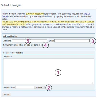
The "Job Identification" section allows the user to provide a job name (default is "my job") and an email address to be used for notification when the job has finished (if you are already logged in this field will be pre-filled). The email provided here also serves as the username by which the job account is identified on the server for accessing results at a later time.
When user account is first created (after the submission of the first job) the user is automatically logged into the server on the machine that is being used. If the login from a previous session has expired or the account needs to be accessed from a different machine, the user needs to go to the server front page http://raptorx.uchicago.edu/StructurePrediction and supply the account email in the login field on the right. After submission of the form the server will send an email to the provided email address with a hyperlink to the page containing the jobs for the account.
The "Sequences for Prediction" section is where the user submits one or more sequences in FASTA format. The sequence(s) can either be supplied by copy-and-pasting into the text box or by uploading a flat text file containing the data.
After the "Submit" button is pressed the user will be redirected to a page of pending and finished jobs for the account used. Please note that each user can have no more than 20 sequences pending prediction at any point in time and a single job can contain at most 10 sequences.
3. Monitoring Job Status and Availability
After submitting the sequence(s), the user will be redirected to the status page of the submitted job similar to the one shown below. This page can be accessed at any time by loggin into the server and clicking "My Jobs" in the menu at the top of the page. For login instructions please refer to Section 2 of this document.
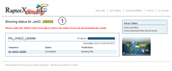
Here, the status of each prediction in the job is given along with overall information of the predictions being done for each submitted sequence. To track the job status in real-time simply refresh the page and the status of the prediction submitted for each sequence in a job will be updated. Clicking on a sequence name will take the user to the result page for this sequence.
4. Interpreting Results
After a job is completed, clicking on a sequence link will take the user to a page similar to one displayed below.
Prediction for the secondary structure classes can be accessed by clicking the link named "Structure labeling for the whole sequence"2. A more detailed description of secondary structure results is given in section 4a.
Our 3D structure predictor explores whether the target sequence appears to consist of multiple domains or is a single folding unit. If multiple domains are found the results are displayed separately for each domain. The sequence partition into domains can be seen in the box labeled "Input Sequence and Domain Partition" on top of the page1. In this box the sequence is shown followed by a row of numbers(or letters in case more than 9 domains where identified) which indicate the domain to which the corresponding residue belongs. Here, 0 indicates absence ofa domain assignment. The results for each domain can be accessed by clicking the links corresponding to specific domains3 (domain limits within a sequence are shown in parentheses). A more detailed description of 3D structure results is given in section 4b.
4a. Interpreting Results - Secondary Structure
After the job has been completed clicking on a secondary structure job in the overview will display a summary page similar to the one depicted below (the numbers used in superscript in this section correspond to the labels in the figure).
Our server currently provides 4 secondary structure predictions:
- 3-class secondary structure
- 8-class secondary structure
- Disorder prediction
- Solvent accessibility prediction
You can switch between the four modes using the blue tab-menu1.
Hovering over a residue will display the exact distribution of secondary structure classes in a popup box appearing next to the residue2. The legend for the color-coding of the structure classes can be found in the right-hand column5.
In addition, the right-hand column provides information on the status of the prediction job3 and links for downloading the prediction results which include the full class distributions for the four models4.
4b. Interpreting Results - Tertiary Structure
Clicking on a domain result link in the overview page will display a summary page similar to the one depicted below (the numbers in superscript used in this section correspond to the labels in the figure).
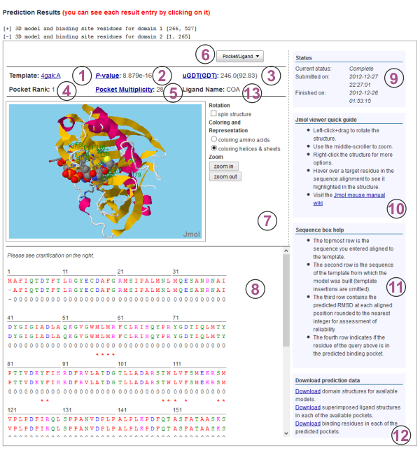
For binding site predictions, a protein structure is built from the top-ranked template chosen from alignment of the target sequence and the structures in the template library. In cases where multiple domains are found, a structure is built and the binding site predictions are made for each domain. The domain assignment of each residue can be seen at the top of the summary page under the input sequence string. The PDB code of the top-ranked template for the structure model is indicated under Prediction Results of each available domain in the top left corner1. Clicking the PDB code of the top-ranked template will take the user to the structure record at the Protein Data Bank http://www.pdb.org.
The P-value2, uGDT and GDT3 of the query alignment with the top ranked template are presented to be used as assessment of the quality of the resulting model structure. The uGDT is the unnormalized GDT (Global Distance Test) score defined as 1*N(1)+0.75*N(2)+0.5*N(4)+0.25*N(8), where N(x) is the number of residues with the local RMSD smaller than x. GDT is calculated as uGDT divided by the domain length and multiplied by a 100.
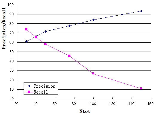
Pocket Multiplicity5 represents the frequency with which the selected pocket was found in the template structures. Figure C depicts the recall/precision of RaptorX-Binding using pocket multiplicity (Ntot in the figure) as a predictor of binding pockets, tested on the 251 binding site benchmark. As we can see from from the figure, when pocket multiplicity is above 40, there is a good chance that the predicted pocket is true.
For an interpretation of the alignment p-value we can consult the following two figures derived from CASP10 official domain threading results. Here, uGDT is calculated between the native structure and the model built from the top-ranked template. From Figure A it can be seen that for values of -log(p-value) greater than 4, 95% of the models have uGDT greater than 50. On the other hand, if for values of -log(p-value) less than 4, 98% of the models have uGDT less than 50. This indicates that if a model has uGDT greater than 50, it can be considered reasonably good. Figure B is an inset of Figure A illustrating the region with uGDT < 100 and -log(p-value) < 6.
Figure A:
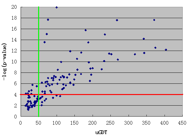
Figure B:
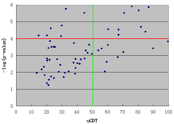
Figure C:
By clicking "Pocket/Ligand" button6 the user can select a pocket and a ligand to visualize with the predicted structure in the Jmol viewer loaded underneath. The pockets are listed in order of their likelihood of being a binding site. Similarly, ligands are listed in order of their likelihood of binding the query protein. After the selection is made, the pocket rank4 and the ligand name13 are displayed above the Jmol viewer. The residues within the pocket are depicted using "ball-and-stick" representation for easy identification. Using the mouse the user can rotate and zoom on the structure. To the right of the structure viewer a menu for controlling the representation of the currently selected structures is available7. Right-clicking the model will bring up a menu of further options for changing the visualization.
The alignment of the target and template sequence used for constructing the 3D model is displayed below the Jmol viewer8. Each position in the alignment is color-coded according to the chemical nature of the residue. The scheme used is: Red=Hydrophobic, Blue=Acidic, Magenta=Basic, Green=Hydroxyl+Amine. Template insertions are omitted. The next row contains the predicted RMSD at each aligned position rounded to the nearest integer as indicators of reliability. In the last row, a '*' under a target residue signifies a predicted binding residue in the selected pocket. Hovering over aligned residues will highlight the target residue in the Jmol viewer.
The right-hand column provides information on the status of the prediction job9, a brief user's guide for the Jmol viewer10 and the sequence box11 as well as links for downloading the prediction results12. The results available for download include the PDB files of the constucted 3D models for each domain, the ligand PDB files rotated to their putative binding poses with the protein structure, grouped into sets according to their predicted pockets, as well as files containing the binding residues for each predicted pocket.